
[Paper Review] DDPM: Denoising Diffusion Probabilistic Models 논문 리뷰
업데이트:
- Paper: Denoising Diffusion Probabilistic Models (Arxiv 2020): arxiv, code, project page
Diffusion Probabilistic Models
- data에 임의의 noise를 더해준 후(forward process), noise를 제거하는 과정(reverse process)을 학습하는 모델
- forward process (diffusion process): data에 noise를 추가하는 과정으로, markov chain을 통해 점진적으로 noise를 더해나간다.
- reverse process: gaussian noise에서 시작하여 점진적으로 noise를 제거해가는 과정
1. DPM
- Paper: Deep Unsupervised Learning using Nonequilibrium Thermodynamics (2015): arxiv
딥러닝에서 현실의 복잡한 dataset을 확률분포 probability distribution로 표현하는 것은 매우 중요하다. 특히 우리가 이 확률분포를 구하고자 할 때에는 tractability와 flexibility라는 개념이 중요한데, 이는 서로 trade-off 관계에 있기 때문에 이 둘을 동시에 만족하긴 어렵다. (복잡한 data에 대해서도 잘 fitting이 되어 있으면서도 계산이 용이한 분포를 찾긴 어려움)
- tractability: Gaussian이나 Laplace distribution 처럼 data에 쉽게 fitting되어 분석이 쉬우며 계산이 용이한 분포
- flexibility: 임의의 복잡한 data에 대해서도 적용이 가능한 분포
Diffusion Probability Model
- extreme flexibility in model structure
- exact sampling
- easy multiplication with other distributions, e.g. in order to compute a posterior, and
- the model log likelihood, and the probability of individual states, to be cheaply evaluate
초창기 Diffusion Probability Model(2015)에서는 diffusion 과정을 통해 우리가 잘 알고있는 distribution (ex. Gaussian)을 target data distribution으로 변환해주는 markov chain을 학습시켜 flexible하면서도 tractable한 distribution을 구하고자 하였다.
2. Diffusion Model
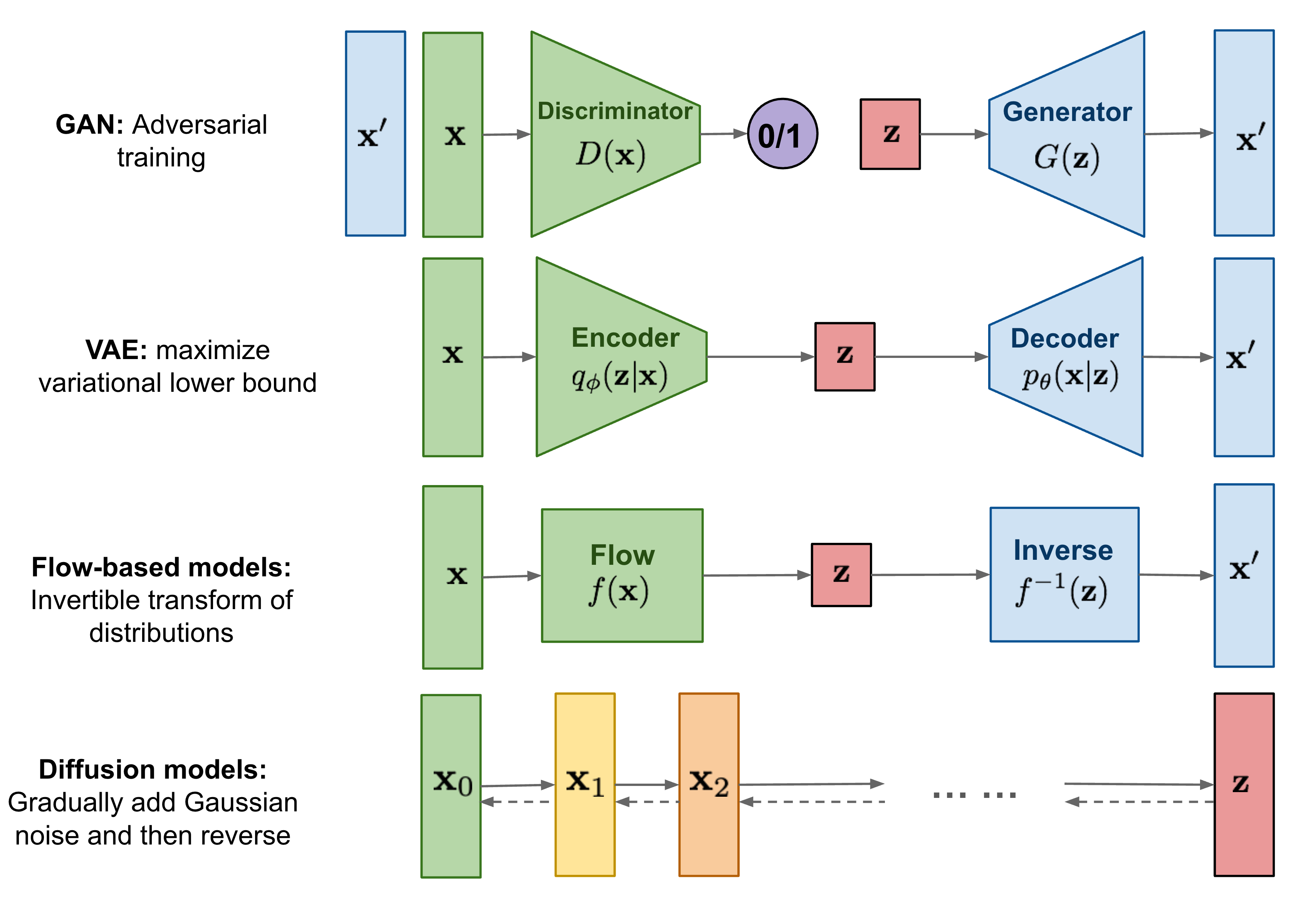
출처: https://lilianweng.github.io/posts/2021-07-11-diffusion-models/
VAE는 image를 encoding하는 network와 latent code를 바탕으로 image를 decoding하는 network 모두를 학습하는 반면, Diffusion model은 이미지를 encoding하는 forward process는 fix된 채 image를 decoding하는 reverse process - single network 만을 학습한다.
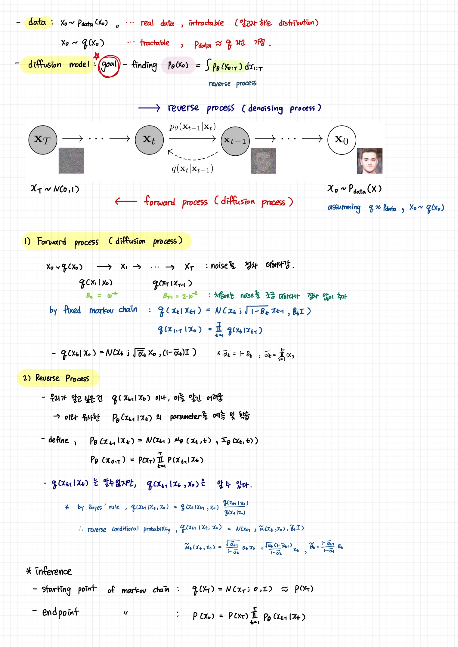
2.1 Forward Process (diffusion process)
- markov chain으로 data에 점진적으로 noise를 추가하는 과정이다 (sampling의 반대방향)
- data에 noise를 추가할 때, variance schedule
를 이용하여 scaling을 한 후 더해준다.
- 매 step마다 gaussian distribution에서 reparameterize를 통해 sample하게 되는 형태로 noise는 추가되는데, 이때 단순히 noise만을 더해주는게 아니라
로 scaling하는 이유는 variance가 발산하는 것을 막기 위함이다.
- variance를 unit하게 가둠으로써 forward-reverse 과정에서 variance가 일정수준으로 유지될 수 있게 된다
- 이 값은 learnable parameter로 둘 수도 있지만, 실험을 해보니 상수로 두어도 큰 차이가 없어서 constant로 두었다고 한다.
- 데이터가 이미지와 비슷할 때에는 이 값을 매우 작게 설정하다가 gaussian distribution에 점점 가까워질 수록 이 값을 크게 설정 (10^-4에서 0.02로 linear하게 증가)
- 매 step마다 gaussian distribution에서 reparameterize를 통해 sample하게 되는 형태로 noise는 추가되는데, 이때 단순히 noise만을 더해주는게 아니라
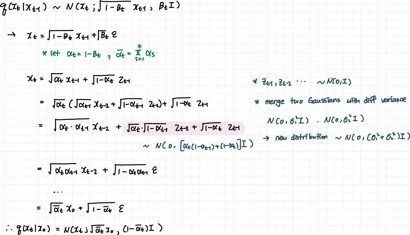
- t번의 sampling을 통해 매 step을 차근차근 밟아가면서
에서
를 만들 수도 있지만, 한번에 이를 할수도 있다.
- 재귀적으로 식을 정리하다보면, 다음과 같은 식이 성립
- 한 step씩 학습을 하면 메모리와 resource가 너무 많이 든다. 그러나 이런식으로 한번에
- 증명
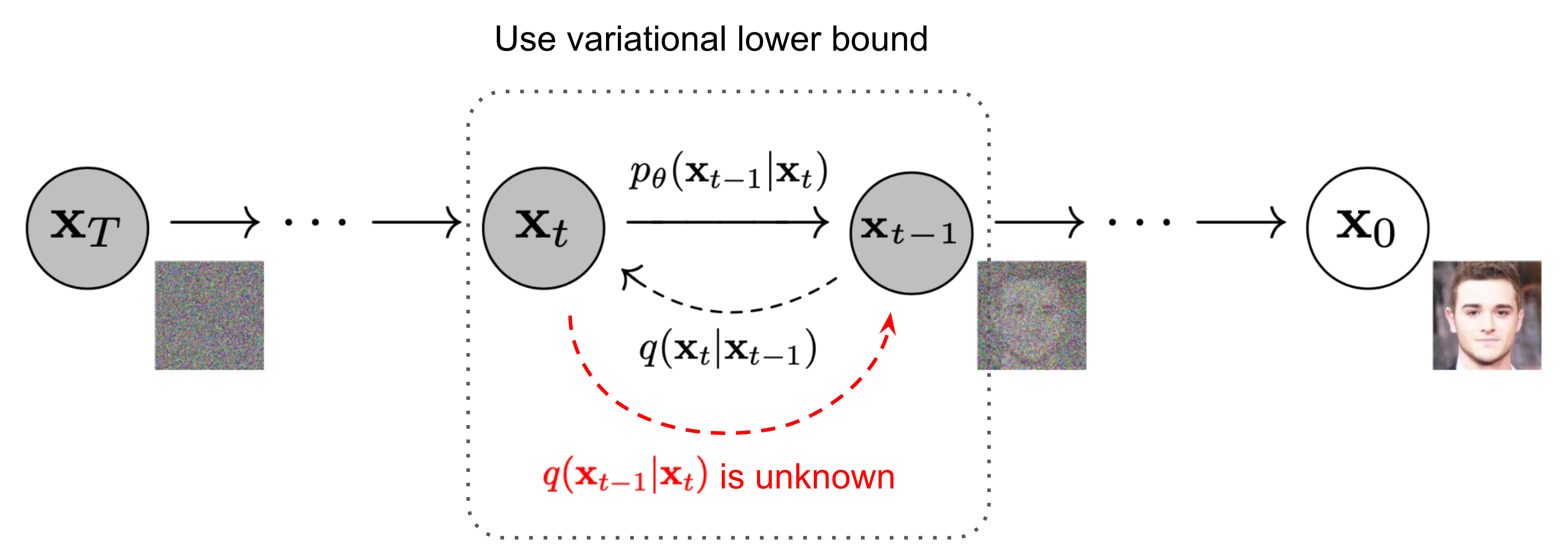
2.2 Reverse Process
- 우리가 학습하고자 하는
reverse diffusion과정- Hierarachical VAE에서의 decoding과정과 비슷
- Gaussian noise
에서 denoising 하면서 이미지
2.3 정리
3. Diffusion models and denoising autoencoders
3.1 Objective Function

여기서 가장 중요한 term은 이다. 우리는
부터 시작하여 conditional하게 식을 전개하다보면,
tractable한 forward process posterior
의 정규분포를 알 수 있는데,
이를 바탕으로 KL divergence를 계산하면 우리가 결과적으로 학습하고자하는
를 학습시킬 수 있다.
3.2 Forward process and 
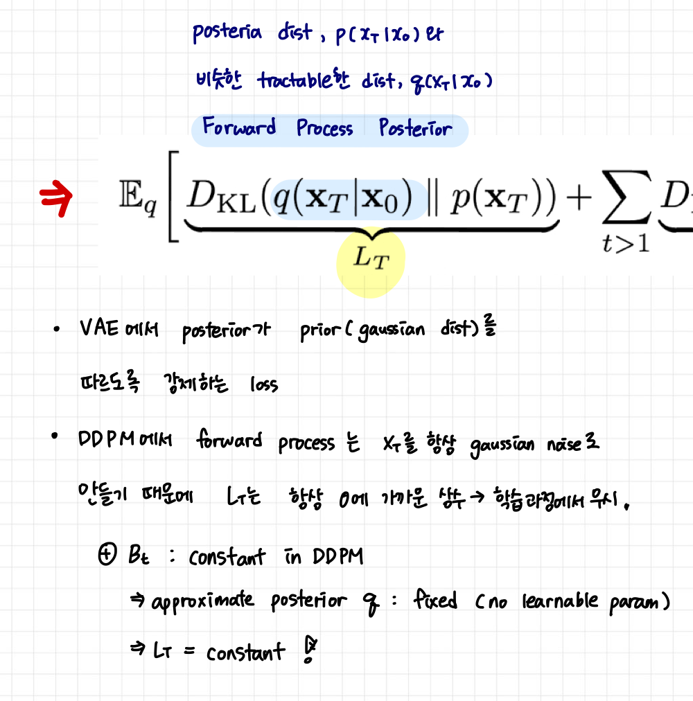
- 위 objective function의 첫번째 term
- DDPM에서의 forward process는
는 prior
와 거의 유사하다. 또한, DDPM에서는 forward process variance
를 constant로 고정시킨 후 approximate posterior를 정의하기 때문에 이 posterior
에는 learnable parameter가 없다.
- 따라서 이 loss term은 항상 0에 가까운 상수이며, 학습과정에서 무시된다.
3.3 Reverse process and 
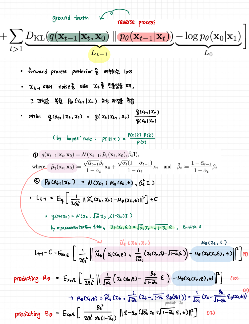
- 위 objective function의 두번째 term
-
이 loss term에서는
(1)
을 예측하도록
the reverse process mean function approximator,를 훈련시켜도 되고
(2)
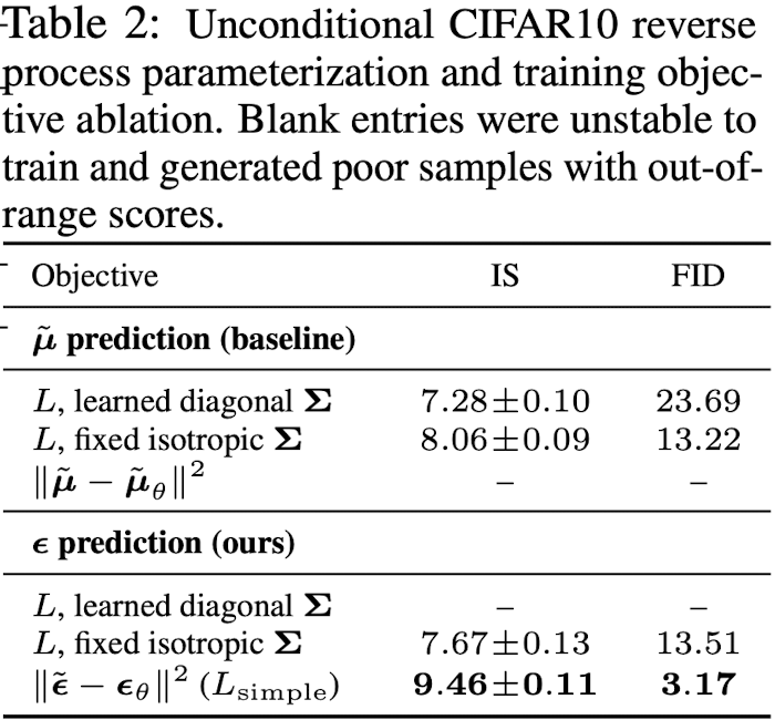
을 예측하도록 학습해도 되는데, 저자들은
ablation study, Table 2)- fixed variances를 사용하는게 더 성능이 좋음
3.4 Data scaling, reverse process decoder, and 
3.5 Simplified training objective
위 objective function에서 중요한 term은 variational bound에 해당하는 과
이다. 저자들은 해당 loss term 을 아래와 같이 simplification 했다고 한다.
- t is uniform between 1 and T
- 위와 같은 simplified objective을 통해 diffusion process를 학습하면 매우 작은 t 에서뿐만 아니라 큰 t에 대해서도 network 학습이 가능하기 때문에 매우 효과적
3.6 Training & Sampling

- Algorithm 1: Training
- noise를 더해나가는 과정, network(
,
)가 t step에서 noise(
-
학습 시에는 특정 step의 이미지가 gaussian noise에서 얼마나 denoising 되었는지를 예측하도록 학습된다.
- noise를 더해나가는 과정, network(
- Algorithm 2: Sampling
- network를 학습하고 나면, gaussian noise에서 시작해서 순차적으로 denoising 하는 것이 가능하다. (by parameterized markovian chain)
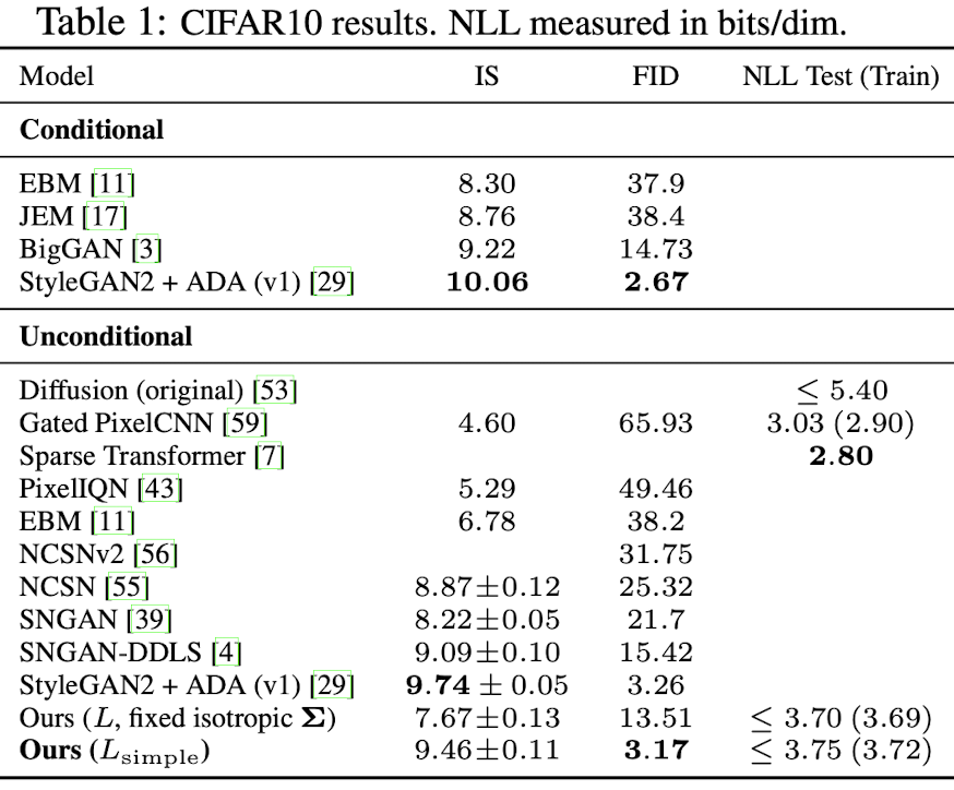
4. Experiments

4.1 Sample quality
댓글남기기