[Paper Review] OSFV(Face vid2vid): One-Shot Free-View Neural Talking-Head Synthesis for Video Conferencing 논문 분석

업데이트: February 17, 2022

Paper: OSFV(face vid2vid): One-Shot Free-View Neural Talking-Head Synthesis for Video Conferencing (CVPR 2021): arxiv, project, unofficial code

OSFV: neural talking-head video synthesis & compression을 할 수 있는 framework

unsupervised 3D keypoint로 person-specific canonical keypoint를 decompose하고 motion-related transformation으로 이 keypoint를 수정

keypoint를 transformation에 따라 다양하게 수정하여 비디오를 생성하므로, user가 자유롭게 view-point를 조절한다거나, 표정을 변화시킬 수 있다.

또한, 본 논문은 기존 모델보다 video compression이 잘된다고 보고한다. (bandwidth가 줄어들 뿐만 아니라 비디오 해상도도 좋아짐)

1. Introduction

neural talking-head video synthesis model
- 본 모델은 이미지로부터 keypoint를 잘 encoding하여 머리를 잘 rotation시킬 뿐만 아니라, neural talking head task에서도 좋은 성능을 보였다.
- source image는 target person의 외형(appearance)를 잘 encoding하며,
- driving video는 output video의 motion을 잘 나타내도록 encoding된다.
one-shot setting
2D-based model
- (장점) 3D graphics-based model에 비해 모델이 가벼우며, 머리, 턱수염 등을 다루기 더 용이하다.
- (한계) 기존 2D-based one-shot talking head model들은 original view point에서만 talking head video 생성이 가능했다. 즉, 다양한 view point에서 이미지를 합성하기가 어렵다.
  
  → 본 모델은 고정된 view point 뿐만 아니라 새로운 local free-view에 대해서도 비디오 합성이 가능!

⭐️ Main Contribution

novel one-shot neural talking-head synthesis approach: 기존 SoTA 모델들보다 더 좋은 성능을 냄

3D graphic model 없이 output video의 Local free-view control이 가능해짐 (다양한 view-point의 비디오 생성이 가능해짐)

video stream에서의 bandwith가 10배 넘게 감소

2. Method

source image: $s$
driving video: $(d_{1}, d_{2}, \ldots, d_{N})$
output video: $(y_{1}, y_{2}, \ldots, y_{N})$
$s=d_1$ 이라면 reconstruction task이고, $s$가 driving video의 프레임이 아니라면 motion transfer task

모델은 크게 3가지 step으로 작동한다.

(a) source image feature extraction
(b) driving video feature extraction
(c) video generation

2D keypoint를 사용하던 FOMM과 다르게 OSFV은 3D keypoint를 사용한다.

keypoint는 unsupervise하게 학습되며 (FOMM과 동일)
facial expression뿐만 아니라 사람의 geometric한 특성을 모델링한다.

2.1 Source image feature extraction

Figure (3)

Appearance feature extractor $F$
- source image $s$ 를 3D apperance feature volume $f_s$ 로 mapping
- 3차원: w, h, d
- 3D feature volume을 잘 모델링해야지 3D space에서 keypoint가 잘 동작하고, 머리가 잘 translation & rotation 될 수 있음
Canonical keypoint detector $L$
- source image로 부터 3D keypoint $x_{c, k} \in \mathbb{R}^{3}$를 추출해주는 모듈
- 저자들은 $K=20$ 으로 두고 실험을 했다고 함
- 일반적인 facial landmark와 다르게 unsupervise하게 학습
- 사람의 geometry signature를 encoding하도록 학습됨
- Unsupervised Learning of Object Landmarks through Conditional Image Generation (NeurlPS 2018)
Head pose estimater network $H$
- source image에서 head pose에 대한 정보를 추정
- parameterized by a rotation matrix $R_{s} \in \mathbb{R}^{3 \times 3}$ and a translation vector $t_{s} \in \mathbb{R}^{3}$
- Hopenet: deep-head-pose (CVPR workshop 2018)
Expression deformation estimator $\Delta$
- K 3D deformation $\delta_{s,k}$ (neutral expression으로 부터 얻어진 keypoint들의 변화)를 추정

위의 모듈들을 통해서 최종적으로 필요한 source keypoint를 구할 수 있다.

$L$ 로부터 얻어진 identity-specific information과 $H, \Delta$ 로부터 얻어진 motion-related information을 이용하여 source 3D keypoint $x_{s,k}$ 를 구함 (이 과정에서 transformation도 진행)

Keypoint computation pipeline

3D keypoint decomposition
- geometry-signatures, head poses, expressions

\[x_{s, k}=T(x_{c, k}, R_{s}, t_{s}, \delta_{s, k}) \equiv R_{s} x_{c, k}+t_{s}+\delta_{s, k}\]

FOMM과 다르게 OSFV는 Jacobian을 추정하지 않는다
- FOMM은 단순히 keypoint의 displacement만을 사용하지 않고 그 주위의 neighbourhood까지 사용할 수 있도록 local affine transformation을 하는데, 이때 Jacobian matrix를 추정하여 비선형 변환인 local affine transformation을 선형으로 근사하곤 했다.
대신 OSFV는 head pose estimator 모듈을 통해 head rotation 정보를 얻곤 하는데, 이 정보가 local patch transformation을 하는데 도움을 준다고 보고한다.
(+) Jacobian 추정을 안하면 비디오 합성시에 transmission bandwidth가 줄어든다고 함

2.2 Driving video feature extraction

OSFV는 supervised 하게 학습이 된다.

source image가 driving image를 모방하도록 학습

따라서 driving image $d$ 로부터 새롭게 canonical 3D keypoint를 뽑지 않고 source image에서 뽑은 정보 $x_{c,k}$ 를 재사용한다.

driving image에서의 3D keypoint source image의 kp와 동일한 방식으로 얻어짐

\[x_{d, k}=T(x_{c, k}, R_{d}, t_{d}, \delta_{d, k}) \equiv R_{d} x_{d, k}+t_{d}+\delta_{d, k}\]

다음과 같이 keypoint는 3D head pose에 따라 자유롭게 transformation 되기 때문에, 우리가 자유롭게 view point를 바꾸고 싶다면 R & t 값을 조절함으로써 비디오를 합성하면 된다.

\[R_{d} arrow R_{u} R_{d} \text { and } t_{d} \longleftarrow t_{u}+t_{d}\]

2.3 Video Generation

source image로부터 K canonical keypoints $x_{c,k}$ 를 구함 (by Canonical keypoint detector $L$)
Head pose estimator $H$ 와 Expression deformation estimator $\Delta$ 의 output 값을 이용하여 source와 driving image의 keypoint를 구함 ⇒ $x_{s,k}, x_{d,k}$
1st order approximation 방식을 이용하여 k개의 keypoint들이 얼마나 warping 되었는지 (warping flow $w_k$ ) 를 계산한다
- source와 driving keypoint $x_{s,k}, x_{d,k}$ 로 부터 K warping flow $w_k$ 를 추정
3에서 얻은 warping flow $w_k$ 정보를 사용하여 source feature volume $f_s$ 를 warping ⇒ $w_K(f_s)$
Motion field estimator $M$ 를 이용하여 $w_K(f_s)$ 로부터 flow composition mask $m$을 추정
- 이 mask는 $K$개의 flows에서 어떤 3D spatial location을 사용할지를 결정
5에서 계산한 Flow composition mask $m$ 을 이용하여 final flow인 composited flow field $w$ 를 구함
Source feature volume $f_s$ 를 final flow인 $w$ 에 따라 warping한 후 ⇒ $w(f_s)$
이 값을 Generator에 넣어 Output image $y$ 를 생성 !

2.3.1 Network Architectures

Motion field estimator $M$
1. kp를 예측한 후에는 예측된 $x_{s,k}, x_{d,k}$를 first-order approximation하여 warping flow map $w_k$ 을 추정한다.
  - $p_d$ 를 driving image $d$ 의 3D feature volume, $p_s$ 를 source image $s$ 의 3D feature volume 라고 하면
  \[w_{k}: R_{s} R_{d}^{-1}(p_{d}-x_{d, k})+x_{s, k} \mapsto p_{s}\]
2. source feature $f_s$ 를 warping: $w_k(f_s)$
3. 3D U-Net 구조인 Motion field estimator에 $w_K(f_s)$ 를 input으로 넣어 flow composition mask $m$을 추정
  - K 3D masks: ${m_{1}, m_{2}, \ldots, m_{K}}$
  \[\sum_{k} m_{k}(p_{d})=1 \text { and } 0 \leqslant m_{k}(p_{d}) \leqslant 1 \text { for all } p_{d}\]
4. the final warping map $w$ 를 구성
  \[\sum_{k=1}^{K} m_{k}(p_{d}) w_{k}(p_{d})\]
5. 2D occlusion mask도 같이 구해놨다가 나중에 Generator의 input으로 사용
Generator: warped 3D apearance features $w(f_s)$ 를 projection해서 2D image로 변환

2.4 Training

train the network: $F, \Delta, H, L, M, G$

2.4.1 Loss function

\[\begin{aligned} \mathcal{L}=& \lambda_{P} \mathcal{L}_{P}(d, y)+\lambda_{G} \mathcal{L}_{G}(d, y)+\lambda_{E} \mathcal{L}_{E}(\{x_{d, k}\})+\\ & \lambda_{L} \mathcal{L}_{L}(\{x_{d, k}\})+\lambda_{H} \mathcal{L}_{H}(R_{d}, \bar{R}_{d})+\lambda_{\Delta} \mathcal{L}_{\Delta}(\{\delta_{d, k}\}) \end{aligned}\]

where λ’s are the weights and are set to 10, 1, 20, 10, 20, 5 respectively in our implementation.

output image가 ground truth와 비슷하도록 만들어주는 loss
- Perceptual Loss $\mathcal{L}_{P}$
  - driving image와 output image간의 p-loss
  - FOMM과 동일하게 multi-scale implementation을 사용
    - Additionally we propose to use this loss on a number of resolutions, forming a pyramid obtained by down-sampling Dˆ and D, similarly to MS-SSIM [39, 32]. The resolutions are 256 × 256, 128 × 128, 64 × 64 and 32 × 32. There are 20 loss terms in total. (FOMM 논문 3.3)
  - VGG pre-trained network로 output image와 ground truth의 feature map을 추출한 후, feature 간의 L1 distance를 계산 → 각 이미지들을 (output, GT) downsampling한 다음에 다시 feature map으로 L1 dis 계산
    - 이렇게 multiple image resolution에 대해 loss 계산을 3번 반복
  - pretrained face VGG network로 single-scale perceptual loss를 계산한 후 final p-loss에 더해줌
- GAN Loss $\mathcal{L}_{G}$
  - multi-resolution patch GAN을 사용
    - discriminator가 patch level에서 predict
    - patch GAN의 hinge loss
  - 추가적으로 discriminator feature matching loss를 도입했다고 함
  - 2 scale의 discriminator
    - single-scale discriminator: 256x256
    - two-scale discriminator: 512x512
keypoint들이 consistent 하고 정확하게 뽑히도록 학습하는 loss
- Equivariance loss $\mathcal{L}_E$
  - image specific keypoints $x_{d,k}$ 가 consistent 하도록 보장하는 loss
  - image $d$ 가 2D transformation을 된다면 $T(d)$ , predicted keypoint $x_d$ 역시 동일하게 transform이 되어야 한다. $x_{T(d)}$이
    - 이러한 성질을 이용하여 본 논문에서는 $L_1$ loss를 걸어줌
    \[\|x_{d}-\mathbf{T}^{-1}(x_{\mathbf{T}(d)})\|_{1}\]
  - 본 논문에서는 2D keypoint가 아니라 3D kp를 사용하기 때문에 loss를 계산하기 전에 이미지 plane에 keypoint를 orthographic projection을 했다고 함
    - 단순히 $z$ values를 drop
- Keypoint prior loss $\mathcal{L}_L$
  - image-specific kp $x_{d,k}$ 가 국소적인 부분에 모여있지 않도록 keypoint를 펼쳐주는 loss
  - 각 keypoint사이의 거리가 멀어지도록 하는 부분
    - keypoint pair의 거리가 일정 threshold $D_t$ 보다 커지면 패널티
  - 평균 depth가 target value $z_t$ 와 비슷하도록 loss
  \[\mathcal{L}_{L}=\sum_{i=1}^{K} \sum_{j=1}^{K} \max (0, D_{t}-\|x_{d, i}-x_{d, j}\|_{2}^{2})+\|Z(x_{d})-z_{t}\|\]
  - 저자들은 $D_t=0.1, z_t=0.33$ 으로 두고 실험했다고 함
Head pose와 keypoint가 잘 학습되도록 돕는 loss
- Head pose loss $\mathcal{L}_H$
  - head rotation $R_d$ 이 ground truth $\bar{R}_d$ 와 비슷하도록 강제하는 loss
    - 이때 $\bar{R}_d$는 pre-trained deep head pose로 inference된 값
  \[\mathcal{L}_{H}=\|R_{d}-\bar{R}_{d}\|_{1}\]
- Deformation prior loss $\mathcal{L}_D$
  - expression deformation $\delta_{d,k}$ 는 canonical keypoint의 편차(deviation)이기 때문에 너무 크면 안된다.
  - 이 값이 작도록 강제하는 loss (L1 norm)
  \[\mathcal{L}_{\Delta}=\|\delta_{d, k}\|_{1}\]

3. Experiments

3.1 Datasets

VoxCeleb2
- 1M talking-head video
- train: 280K videos
- validation: 36K
TalkingHead-1KH
- 저자들이 직접 모은 large-scale talking head video datasets (1000hours)
- 추가로 Ryerson audio-visual dataset의 비디오도 사용했다고 함
- 180K videos
- Vox2보다 화질도 좋고 용량도 크다고 함 (저자들이 해상도와 bit-rate가 높은 영상들만 추려서 사용했다고 함)

3.2 Talking-head image synthesis

3.2.1 Baseline

FOMM: First Order Motion Model for Image Animation (NeurIPS 2019) : arxiv, code, review
fs vid2vid: Few-shot Video-to-Video Synthesis (NeurlPS 2019): arxiv, project, code
Bi-layer model: Fast Bi-layer Neural Synthesis of One-Shot Realistic Head Avatars (ECCV 2020): arxiv, project, code, review
- bi-layer model은 배경 예측을 못해서 배경을 빼고 quantitative analyses
bi-layer는 pre-trained model을 이용하고 FOMM이랑 fs vid2vid 은 scratch부터 학습했다고 함

3.2.2 Metrics

reconstruction faithfulness: L1, PSNR, SSIM/MS-SSIM
- L1: GT랑 recon image간의 average L1 dist
- PSNR: GT랑 recon image간의 MSE를 계산 → image recon quality 측정
- SSIM/MS-SSIM: structural similarity between pataches of the input images를 계산 → PSNR보다 좀더 global illumination changes에 robust 함
output visual quality: FID
- OSFV 모델을 통해 생성한 비디오가 얼마나 original video처럼 진짜같을지
- FID: pre-trained Inception V3 network를 사용해서 GT와 recon image의 feature를 뽑고 distance를 계산
semantic consistency: AKD(average keypoint distance)
- original video에서 뽑힌 landmark랑 생성된 비디오의 landmark가 얼마나 유사한지
- facial landmark detector를 사용해서 landmark간의 average distance를 구함

3.2.3 Same-identity reconstruction

source image와 driving image를 같은 사람으로 두고 s가 d를 recon하도록 실험

성능 짱 좋음
OSFV 모델은 학습해야하는 parameter가 많은 무거운 모델인데, 저자들은 단순히 모델이 커서 성능이 잘 나온게 아니라는 걸 증명하려고 FOMM-L와도 비교실험했다고 함
- FOMM-L: FOMM보다 filter size가 2배나 큰 모델

3.2.4 Cross-identity motion transfer

source와 drive image간의 identity가 다른 경우에도 source image가 drive image의 정보를 잘 모사하도록 비디오가 생성이 되는지

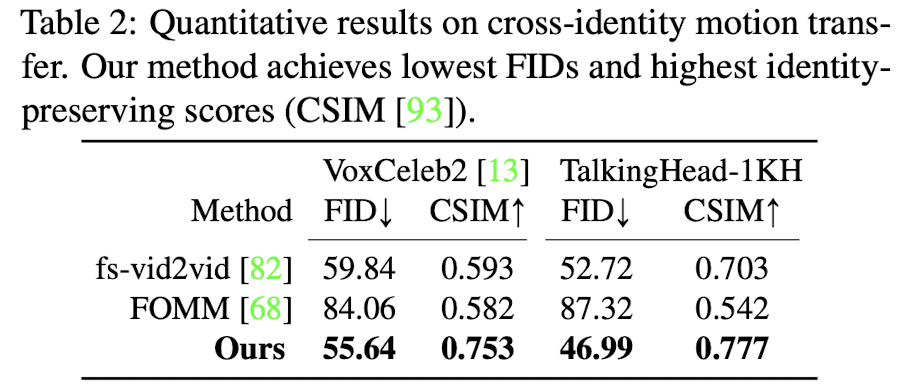
잘됨

3.2.5 Relative motion transfer

(Two-step vs direct) keypoint prediction
- 현재 OSFV 모델은 keypoint 예측을 two-step으로 함
  1. canonical keypoint 예측 → $x_{c,k}$
  2. transformation & deformation 적용 → source kp, drive kp $x_{s,k}, x_{d,k}$
- 한번에 바로 keypoint를 뽑을 수는 없을까?
  - 저자들은 이미지로부터 바로 source kp, drive kp를 예측하는 network를 학습 시켜봤다고 한다.
    - 표준 kp인 $x_{c,k}$ 를 예측하지 않고, 바로 source kp, drive kp $x_{s,k}, x_{d,k}$ 를 예측
    - 즉, Pose estimator $H$ 와 deformation estimator $\Delta$ 가 필요 없음
      - 기존 two-step 방식은 transformation & deformation 정보를 얻기 위해 Pose estimator $H$ 와 deformation estimator $\Delta$ 가 필요했었음
  - (결과) 정량적으로도 성능이 안좋으며, head pose에 대한 정보를 encoding하지 않기 때문에 pose control이 안된다.

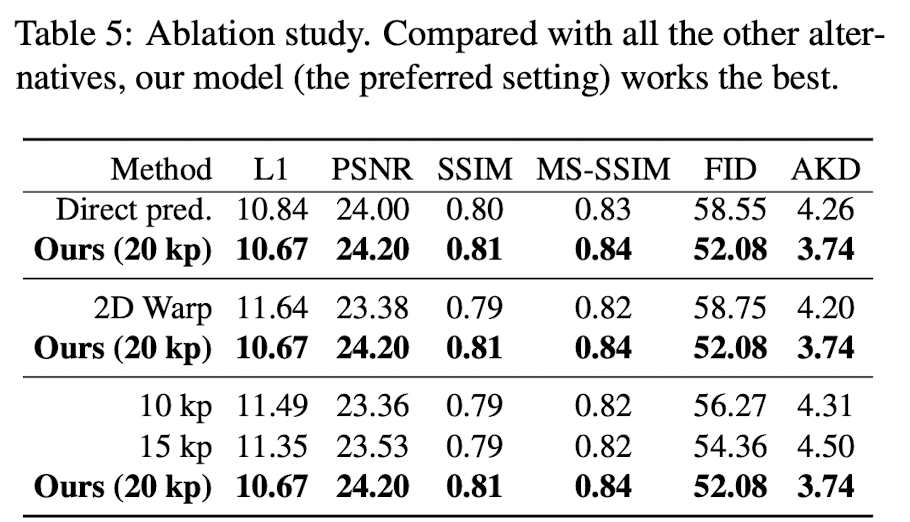
(3D vs 2D) warping
- 저자들은 예측된 keypoint를 바탕으로 3D feature를 warping해서 3D flow field를 생성하곤 했는데, 이를 2D field에서도 실험해봤다고 한다.
- table 5 참고
Number of keypoints
- kp도 다양하게 실험해봤는데, 20개가 best
- table 5 참고

3.2.6 Failure cases

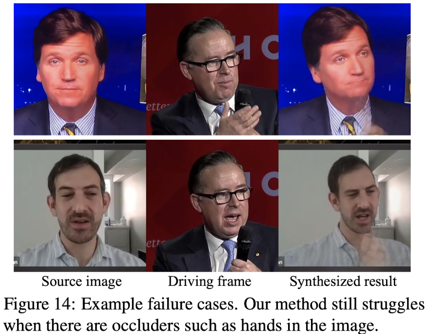
Fig 14 처럼 손이나 어떤 object가 얼굴을 가리고 있는 경우 synthesis quality가 현저히 떨어짐
추가로 실패 케이스들이 존재

3.2.7 Canonical keypoints for face recognition

Canonical keypoint는 pose와 expression 변화와는 무관하게 얼굴의 shape(눈,코,입)과 같은 사람의 geometry signature을 encoding하도록 훈련된다.
저자들은 이 canonical keypoint가 얼마나 face recognition을 잘하는지 확인해보았다고 한다.
random으로 kp를 뽑을 때 보다 27배 더 좋은 성능을, landmark detector보다 5배 더 좋은 성능을 보였다고 한다.

3.3 Face redirection

저자들은 얼굴의 방향을 바꿀 수 있는지도 실험을 했다고 함

Baselines
- pSp (pixel2style2pixel): original image를 latent space로 projection한 다음에 pre-trained StyleGAN으로 정면의 이미지를 생성
- RaR (Rotate-and-Render): 3D face model을 이용하여 input image를 다른 pose로 re-rendering
Metrics: 2가지에 대해 평가
1. identity preservation
  - pre-trained face recognition network 사용
  - rotated face와 original face 사이의 거리를 계산
2. head pose angles
  - pre-trained head pose estimator를 통해 회전된 face의 head angle을 구하고, 원하는 angle이면 good으로 평가 → good의 ratio 계산

Twitter Facebook LinkedIn

Jihye Back