
[Paper Review] Deep Face Drawing: Deep Generation of Face Images from Sketches 논문 리뷰
업데이트:
Deep Face Drawing: local-to-global approach
- key face component들의 feature embedding을 학습하여 input sketch의 주요 part를 component manifold로 projection
- embedded component feature들을 realistic image로 mapping해주는 deep neural network
기존의 sketch-to-image translation 모델들은 sketch와 image의 pair dataset으로 학습을 했기 때문에 거의 reconstruction task에 가까웠으며, real image의 edge map과 비슷한 sketch를 입력해야 realistic face image 생성이 가능했다.

즉, abstract 한 이미지를 input으로 준다면 이미지 생성이 잘 안된다.
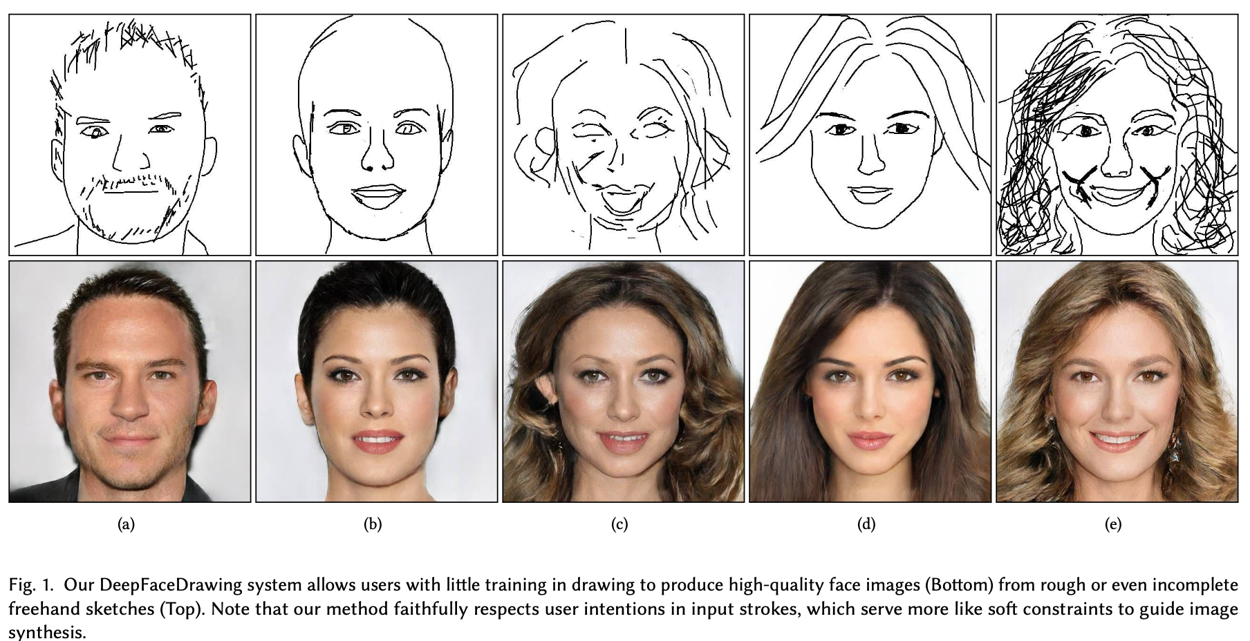
본 논문에서는 대충 그려진 input sketch라도 projection될 수 있는 공간을 implicit하게 학습한다. 얼굴 전체를 global하게 embedding할 수 있는 공간을 학습하려면 high-dimension space가 필요하여 어렵다. 따라서 얼굴의 각 파트들을 나눈 후 이를 각각의 component manifold에 projection한다.
Data Preperation

(b) holistically-nested edge detecthion (HED)
(c) APDrawingGAN
(d) Canny edge detection
- 불연속적인 line들
(e) Photocopy filter in Photoshop
(f) (e)에다가 sketch simplification method 적용
최종적으로는 (f) Photocopy + sketch simplification 방식을 채택하여 CelebAMask-HQ 의 17K paired dataset을 구함
- 16860 training + 842 testing
Architecture

(1) Component Embedding Module (CE)
- face components의 feature embedding을 implicit하게 학습하는 모듈
- 우리는 대충 그려놓은 sketch를 input으로 줄 수 있다. 따라서 이 경우에도 manifold로 projection 될 수 있게 모델을 implicit하게 학습
- sketched face component의 feature vector를 locally linear embedding (LLE) algorithm으로 component manifold에 projection
- component manifold는 locally linear
- face sketch를 5개의 components로 decompose
- left-eye, right-eye, nose, mouth, remainder
Fig 4와 같은 이미지들도 있기 때문에 눈 각각을 따로 처리
- 5개의 auto-encoder network ${E_{c}, D_{c}}$ 를 사용
- 5개의 encoder와 5개의 decoder
- 중간에 FC layer를 추가하여 latent descriptor를
512-dim로 만들었다고 함- latent code의 dimension도 다양하게 실험:
(128, 256, 512) 512-dim: sketch detail을 제일 잘 표현하며 reconstruction도 잘됨128-dim: dimension이 작아질수록 blurry image가 생성
- latent code의 dimension도 다양하게 실험:
- 또한, 오직 conv, deconv로만 encoder, decoder를 구성하지 않고 conv/deconv 연산 후에 residual block을 추가

(2) Feature Mapping Module (FM)
- Problem: CE의 learned decoder를 이용하여 다시 component sketch로 합성된 정보를 이용하면 이미지가 inconsistency하게 생성될 수 있다.
Fig 5(c): 이전 모델들의 방식처럼 이미지를 생성하면 face component들 사이에 misalignment가 생긴다던가, hair style이 incompatible하다던가 하는 여러 artifact들이 생긴다.- 이전 모델들은 input sketch를 hard constraint로 주었기 때문에(정말 정교한 sketch를 input으로 주어 이를 잘 반영하는 image 생성) sketch에 대한 정보를 해석하려 하지 않고, 이를 반영하도록만 이미지가 생성된다.
- 저자들이 이 문제를 관찰해본 결과, 주로 각 component들이 overlapping되는 영역에서 inconsistency 문제가 생겼다고 한다.
- Solution: sampled manifold point의 feature vector의 channel을
1-ch에서32-ch로 확장1-ch는 overlapping region의 neighboring component까지 catch하기엔 부족하여 이를 multi-channel로 확장- information flow가 향상되며 face component간의 inconsistency도 줄어들었다고 한다.
- 각 decoding model은 FC layer와 decoding layer로 구성

(3) Image Synthesis Module (IS)
- FM의 feature map을 합친 결과를 IS module에 넣어 이미지 생성
- conditional GAN architecture
- Generator: pix2pixHD의 global generator처럼 encoder part, residual block, decoding unit으로 구성
- multi-scale Discriminator: by pix2pixHD
Two-stage Training
2-stage로 network를 학습
- Stage-1
- 오직 CE module 만을 학습
- 각 auto-encoder로 sketch component를 feature embedding 할 수 있도록 training 한다
- self-supervised 방식: input sketch와 recon sketch의 MSE loss
- Stage-2
- end-to-end로 FM과 IS module을 학습
- GAN loss와 L1 loss → 생성된 이미지의 pixel-wise quality를 향상
- discriminator에 perceptual loss
Manifold Projection
-
sketch의 각 component들을 trained encoder로 embedding
\[\mathcal{F}^{c}=\{f_{i}^{c}=E_{c}(s_{i}^{c})\}\] -
$\mathcal{F}^{c}$ 는 low-dimensional manifold → $\mathcal{M}^{c}$ 로 space를 변경
- $\mathcal{M}^{c}$ 의 component manifold는 locally linear하기 때문에 비슷하게 생긴 component일수록 가까이 위치한다.
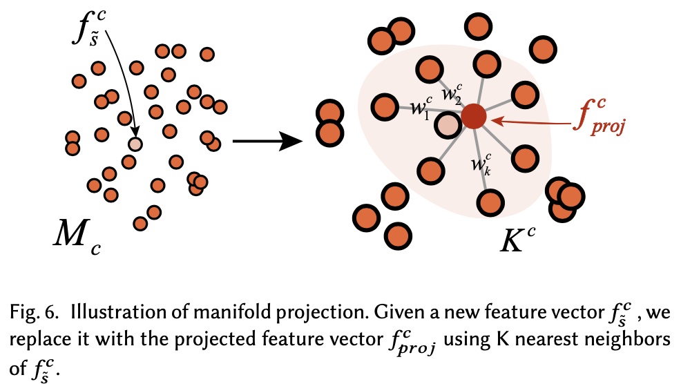
Mapping c-th component feature vector: $f_{\tilde{s}}^{c}$ → $f_{\text{proj}}^{c}$
- Euclidean space에 있는 $\mathcal{F}^{c}$ 에서 $f_{i}^{c}$의 K nearest samples $\mathcal{K}^{c}={s_{k}^{c}} \text { (with }{s_{k}} \subset \mathcal{S} \text { ) }$를 뽑음
- 실험을 해보니 K=10 가 제일 괜찮았다고 함
-
$\mathcal{M}^{c}$의 $\tilde{s}^{c}$를 recon하도록 다음 식을 minimize
\[\min \|f_{\tilde{s}}^{c}-\sum_{k \in \mathcal{K}^{c}} w_{k}^{c} \cdot f_{k}^{c}\|_{2}^{2}, \quad \text { s.t. } \sum_{k \in \mathcal{K}} w_{k}^{c}=1\]- $w_{k}^{c}$ : samples $s_{k}^{c}$ 의 unknown weight
-
$w_{k}^{c}$ 를 알면, projected point of $\tilde{s}^{c} \text { on } \mathcal{M}^{c}$ 는 계산될 수 있다.
\[f_{p r o j}^{c}=\sum_{k \in \mathcal{K}^{c}} w_{k}^{c} \cdot f_{k}^{c}\]- $f_{p r o j}^{c}$: $\tilde{s}^{c}$ 의 feature vector로 FM/IS module의 input

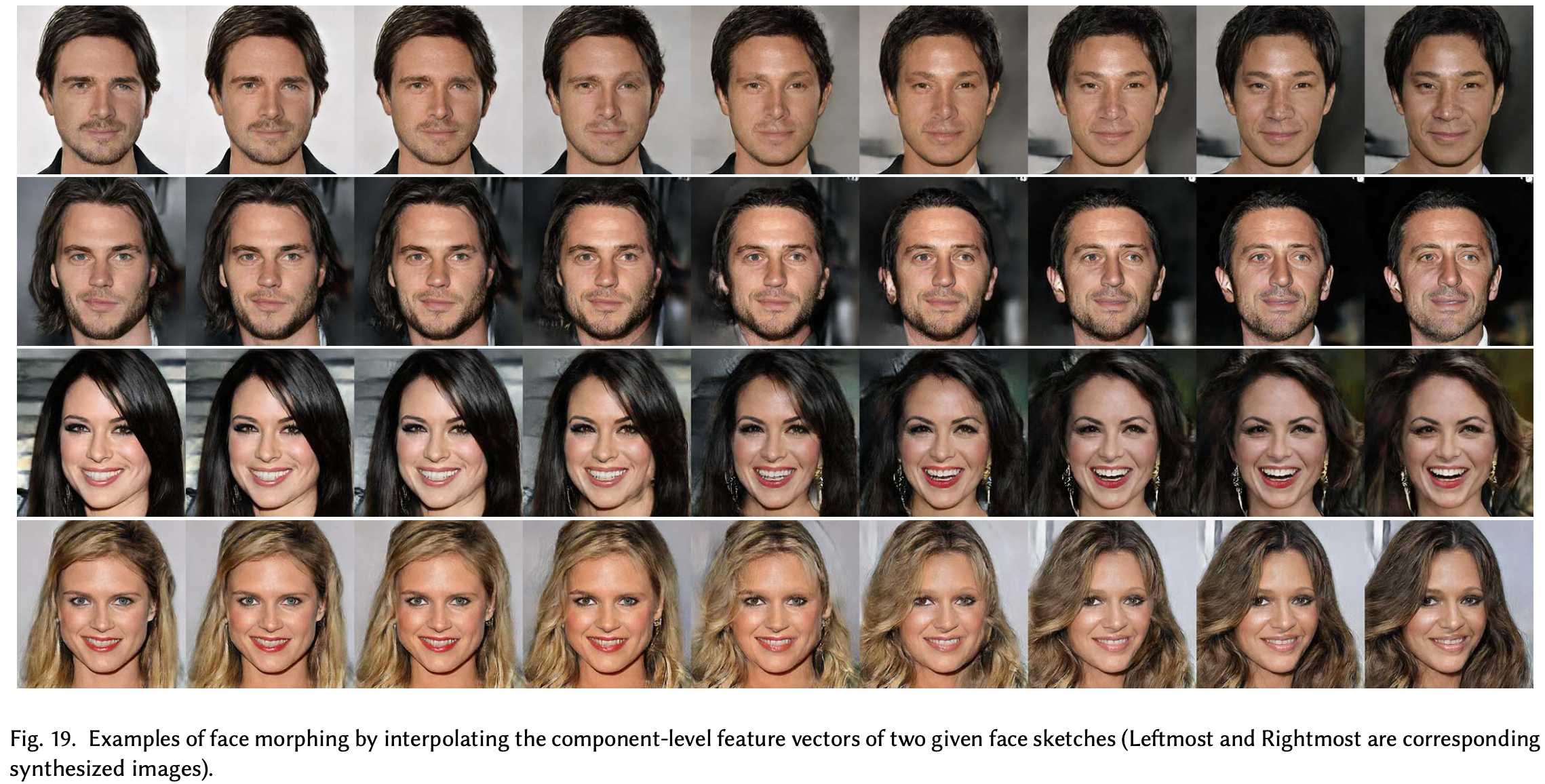
새롭게 정의한 manifold가 정말로 locally linear한지 확인하려고 두 이미지를 random sampling한 후, linear interpolation을 해봤다고 한다. (결과 Fig 7)
Shadow-guided Sketching Interface

-
Fig 8의 왼쪽처럼 shadow로 sketch에 대한 guide를 줌 -
현재 그려놓은 sketch $\tilde{s}$ 가 있을 때, feature space에서 Euclidean distance를 구해 $\tilde{s}^{c}$ 와 비슷한 10개의 sketch component 이미지를 shadow로 그려놓음
- 새로운 input stroke가 그려질 때마다 shadow도 update

Blending feature vector
-
feature vector를 blending 함으로써 본인의 스케치를 얼마나 따를지를 조절할 수 있다.
\[f_{\text {blend }}^{c}=w b^{c} \times f_{\tilde{s}}^{c}+(1-w b^{c}) \times f_{\text {proj }}^{c}\]
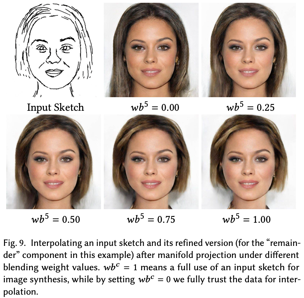

- 각 component 마다 blending 정도를 조절 가능
Result


댓글남기기