
[nlp] Learning Phrase Representations using RNN Encoder-Decoder for Statistical Machine Translation 논문 리뷰 및 코드 실습
업데이트:


2021/03/29 Happy-jihye 🌺
paper : Learning Phrase Representations using RNN Encoder-Decoder for Statistical Machine Translation(2014)
0. Introduction

-
이번 노트북에서는 Learning Phrase Representations using RNN Encoder-Decoder for Statistical Machine Translation(2014) paper의 모델을 간단하게 구현할 예정입니다.
-
이 논문은 두 가지 내용으로 유명합니다. 하나는 기계번역 Neural Machine Translation(NMT) 분야에서 널리 쓰이고 있는 Seq2Seq architecture의 제안이고, 두번째는 LSTM의 대안인 Gated Recurrent Unit(GRU)의 도입입니다.
- 이 논문은 Seq2Seq model을 제시한 논문이지, 이를 NMT 분야에 사용한 논문은 아닙니다. 이 논문에서는 당시 활용되던 Statical Machine Translation(SMT)분야의 한 파트로서 RNN Encoder-Decoder model을 제안하였습니다.
- 실제로 이 모델을 NMT 분야에 적용한 논문은 Sequence to Sequence Learning with Neural Networks입니다.
- SMT vs NMT
-
Sequence to Sequence Learning with Neural Networks, LSTM 등에 대해 공부하고 싶으시다면 이 글들(Seq2Seq-NMT과 Understanding LSTM Network)을 참고하시면 좋을 것 같습니다 :)
1. Paper Review
RNN Encoder-Decoder
이번 시간에 배울 모델의 architecture는 간단합니다.
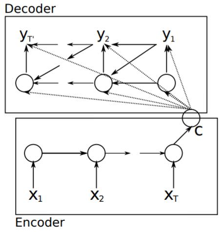
- RNN Encoder-Decoder은 encoder와 decoder 역할을 하는 2개의 Recurrent Neural Network(RNN)으로 구성되어 있으며, Encoder는 가변 길이의
source sequence를 고정된 크기의context vector로 만들고 Decoder는 이context vector를 다시 가변 길이의target sequence로 변환합니다.
context vector는 모든 decoder의 노드들에 관여를 하며, 번역이 문장 단위가 아닌, 단어나 구문 단위로 쪼개서 되기 때문에 이 모델은 통계 기계 번역(Statistical Machine Translation, SMT)를 따른다고 볼 수 있습니다.
즉, RNN Encoder-Decoder는 가변 길이의 input과 output에 대한 조건부 확률을 학습하는 모델이라고 볼 수 있습니다.
\[p(y_1,..,y_{T'}~\vert~x_1,...,x_T)\]Encoder
Encoder은 RNN구조로 되어있으며, 이 구조를 식으로 표현하면 다음과 같습니다.
\[\mathbf{h}_{<t>}=f(\mathbf{h}_{<t-1>},x_t)\]Decoder
Decoder 역시 RNN구조로 되어있습니다. 다만, decoder의 hidden state에서는 이전의 output인 $y_{t-1}$과 encoder의 결과인 context vector를 추가 input으로 받습니다.
\[\mathbf{h}_{<t>}=f(\mathbf{h}_{<t-1>}, y_{t-1}, \mathbf{c})\]output을 조건부 확률로 나타내면 다음과 같이 표현할 수 있습니다.
\[p(y_t\vert y_{t-1}, y_{t-2},...,y_1,\mathbf{c})=g(\mathbf{h}_{<t>},y_{t-1},\mathbf{c})\]- 여기서 $f, g$ 는 softmax와 같은 activation function입니다.
Encoder와 Decoder로 구성된 RNN Encoder-Decoder 는 아래의 식인 conditional log-likelihood를 최대화하는 방향으로 학습됩니다.
- 이때, $θ$는 모델의 parameter를 뜻하고 $(\mathbf{x}_n, \mathbf{y}_n)$는 training data의 input sequence, output sequence 쌍입니다.
GRU (Hidden Unit that Adaptively Remembers and Forgets)
이 논문에서는 RNN Encoder-Decoder model(일명 Seq2Seq)외에도 놀라운 architecture인 GRU를 제시했습니다. 이는 LSTM을 수정한 것으로, LSTM과 비슷한 일을 하지만 연산이 더 간단하며 구조 역시 더 간단합니다.
GRU의 구조를 그림으로 표현하면 다음과 같습니다.
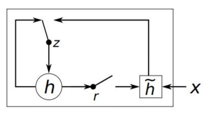
이제부터는 위의 구조에서 hidden unit이 어떻게 활성화되는지를 알아보겠습니다.
첫번째로 reset gate 인 $r_j$는 다음과 같이 계산됩니다.
- 여기서 $W_r, U_r$은 가중치 벡터이며, $σ$는 logistic sigmoid function입니다.
- 이 reset gate의 값이 0에 가까워지면, 이전 hidden state 값이 무시되고 현재의 input만이 hidden state에 영향을 줍니다.
두번째로 update gate 인 $z_j$는 다음과 같이 계산됩니다.
- update gate는 얼마나 많은 정보를 update할지 결정하는 값으로 LSTM의
memory cell과 유사합니다.
우리는 이 두개의 gate를 사용하여 hidden unit의 값을 계산하며, 이는 LSTM과 유사하게 동작을 합니다.
\[\begin{matrix} h_j^{<t>}=z_jh_j^{<t-1>}+(1-z_j)\tilde{h}_j^{<t>}\\ \\ \tilde{h}_j^{<t>}=\phi\big([\mathbf{W}\mathbf{x}]_j+[\mathbf{U}(\mathbf{r}\odot\mathbf{h}_{<t-1>})]_ j \big) \end{matrix}\]Statistical Machine Translation
기존에 흔히 사용되던 통계적 기계 번역 방식은 주어진 문장 $e$ 에 대한 translation function 인 $f$를 찾는 겁니다. 즉, 다음의 식을 최대화하기 위한 식으로 볼 수 있습니다.
하지만 실제 계산에서는 $p(\mathbf{f}\vert\mathbf{e})$ 보다 $log p(\mathbf{f}\vert\mathbf{e})$를 최대화 하는 것이 쉬우므로 다음의 식을 최대화합니다.
\[\log p(\mathbf{f}\vert\mathbf{e})=\sum^N_{n=1}w_n f_n(\mathbf{f},\mathbf{e})+\log Z(\mathbf{e})\]- 여기서 $f_n$ 은 n번째 feature이며, $w_n$ 은 가중치 입니다. 각 가중치는 BLEU score를 최대화하는 방향으로 학습됩니다.
- $Z(e)$ 는 normalization 상수입니다.
2. Code Practice
Preparing Data
!apt install python3.7
!pip install -U torchtext==0.6.0
!python -m spacy download en
!python -m spacy download de
import torch
import torch.nn as nn
import torch.optim as optim

from torchtext.datasets import Multi30k
from torchtext.data import Field, BucketIterator

import spacy
import numpy as np

import random
import math
import time

SEED = 1234

random.seed(SEED)
np.random.seed(SEED)
torch.manual_seed(SEED)
torch.cuda.manual_seed(SEED)
torch.backends.cudnn.deterministic = True
Tokenizers
- tokenizers는 문장을 개별 token으로 변환해주는 데 사용됩니다.
- e.g. “good morning!” becomes [“good”, “morning”, “!”]
- nlp를 쉽게 할 수 있도록 도와주는 python package인
spaCy를 이용하여, token화를 할 예정입니다.
spacy_de = spacy.load('de')
spacy_en = spacy.load('en')
def tokenize_de(text):
  return [tok.text for tok in spacy_de.tokenizer(text)]

def tokenize_en(text):
  return [tok.text for tok in spacy_en.tokenizer(text)]
다음으로는 Field 라이브러리를 사용하여 데이터를 처리합니다.
SRC = Field(tokenize= tokenize_de,
            init_token = '<sos>',
            eos_token = '<eos>',
            lower = True)

TRG = Field(tokenize= tokenize_en,
            init_token = '<sos>',
            eos_token = '<eos>',
            lower = True)
- dataset으로는 Multi30k dataset을 사용하였습니다. 이는 약 3만개의 영어, 독일어, 프랑스어 문장이 있는 데이터이며 각 문장 당 12개의 단어가 있습니다.
exts는 source와 target으로 사용할 언어를 지정합니다.
train_data, valid_data, test_data = Multi30k.splits(exts= ('.de', '.en'),
                                                    fields = (SRC, TRG))
downloading training.tar.gz
training.tar.gz: 100%|██████████| 1.21M/1.21M [00:01<00:00, 705kB/s]
downloading validation.tar.gz
validation.tar.gz: 100%|██████████| 46.3k/46.3k [00:00<00:00, 174kB/s]
downloading mmt_task1_test2016.tar.gz
mmt_task1_test2016.tar.gz: 100%|██████████| 66.2k/66.2k [00:00<00:00, 159kB/s]
print(f"Number of training examples: {len(train_data.examples)}")
print(f"Number of validation examples: {len(valid_data.examples)}")
print(f"Number of testing examples: {len(test_data.examples)}")
Number of training examples: 29000
Number of validation examples: 1014
Number of testing examples: 1000
print(len(vars(train_data.examples[0])['src']))
print(len(vars(train_data.examples[1])['src']))

print(vars(train_data.examples[0]))
print(vars(train_data.examples[1]))
13
8
{'src': ['zwei', 'junge', 'weiße', 'männer', 'sind', 'im', 'freien', 'in', 'der', 'nähe', 'vieler', 'büsche', '.'], 'trg': ['two', 'young', ',', 'white', 'males', 'are', 'outside', 'near', 'many', 'bushes', '.']}
{'src': ['mehrere', 'männer', 'mit', 'schutzhelmen', 'bedienen', 'ein', 'antriebsradsystem', '.'], 'trg': ['several', 'men', 'in', 'hard', 'hats', 'are', 'operating', 'a', 'giant', 'pulley', 'system', '.']}
Build Vocabulary
build_vocab함수를 이용하여 각 token을 indexing해줍니다. 이때, source와 target의 vocabulary는 다릅니다.min_freq를 사용하여 최소 2번 이상 나오는 단어들만 vocabulary에 넣어주었습니다. 이때, 한번만 나오는 단어는<unk>token으로 변환됩니다.- 이때, vocabulary는 training set에서만 만들어져야합니다. (validation/test set에 대해서는 만들어지면 안됨!!)
SRC.build_vocab(train_data, min_freq = 2)
TRG.build_vocab(train_data, min_freq = 2)
print(f"Unique tokens in source (de) vocabulary: {len(SRC.vocab)}")
print(f"Unique tokens in target (en) vocabulary: {len(TRG.vocab)}")
Unique tokens in source (de) vocabulary: 7855
Unique tokens in target (en) vocabulary: 5893
Create the iterators
BucketIterator를 이용하여 batch size별로 token들을 묶고, 어휘를 읽을 수 있는 token에서 index로 변환해줍니다.
# for using GPU
device = torch.device('cuda' if torch.cuda.is_available() else 'cpu')
BATCH_SIZE = 128

train_iterator, valid_iterator, test_iterator = BucketIterator.splits(
    (train_data, valid_data, test_data),
    batch_size = BATCH_SIZE,
    device = device
)
- 다음은 batch size가 무엇인지에 대해 이해해보기 위해 첫번째 batch를 출력해본 예제입니다.
BucketIterator를 통해 batch끼리 묶으면 [sequence length, batch size]라는 tensor가 생성되며, 이 tensor는 train_data를 batch_size로 나눈 결과값만큼 생성됩니다.- 이 예제에서는 128의 크기를 가진 batch가 총 227개 생깁니다.
- 또한, batch에서
sequence length는 그 batch 내의 가장 긴 문장의 길이로 결정되며 그보다 짧은 문장들에 대해서는<pad>token으로 남은 tensor값이 채워집니다.
print(TRG.vocab.stoi[TRG.pad_token]) #<pad> token의 index = 1

for i, batch in enumerate(train_iterator):
    src = batch.src
    trg = batch.trg

    src = src.transpose(1,0)
    print(f"첫 번째 배치의 text 크기: {src.shape}")
    print(src[0])
    print(src[1])

    break

print(len(train_iterator))
print(len(train_iterator)*128)
1
첫 번째 배치의 text 크기: torch.Size([128, 33])
tensor([   2,    8,   67,  217,   12,   33,  214,    9,   35,   17,  101,   17,
         998,   20, 1787,   93,    4,    3,    1,    1,    1,    1,    1,    1,
           1,    1,    1,    1,    1,    1,    1,    1,    1], device='cuda:0')
tensor([  2,  43,  41,  57, 215,   9,  14,   7, 555,   9,  18, 101,   7, 234,
          9,  22, 354,  14, 337, 119,  69,   4,   3,   1,   1,   1,   1,   1,
          1,   1,   1,   1,   1], device='cuda:0')
227
29056
Building the Seq2Seq Model
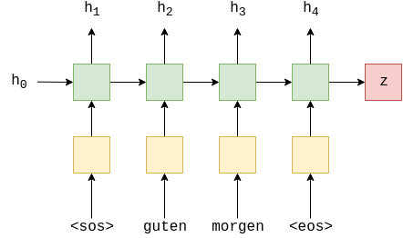
Encoder
-
Encoder는 1개의 GRU layer로 구성되어 있습니다. LSTM과는 달리 GRU에서는 각 dropout이 RNN의 각 layer간에 사용되기 때문에 dropout을 GRU의 인수로 주지 않아도 됩니다.
-
또한, GRU는 LSTM과 달리 cell state를 RNN network의 입출력으로 사용하지 않습니다.
$h_t = \text{GRU}(e(x_t), h_{t-1})$
$(h_t, c_t) = \text{LSTM}(e(x_t), h_{t-1}, c_{t-1})$
$h_t = \text{RNN}(e(x_t), h_{t-1})$
-
Encoder의 최종식을 표현하면 다음과 같습니다.
$h_t = \text{EncoderGRU}^1(e(x_t), h_{t-1})$
-
마지막 RNN을 거치고 나면, context vector인 $z=h_T$를 얻게 됩니다.
- GRU는 LSTM과 비슷한 성능을 내지만, 메모리를 보다 효율적으로 사용할 수 있는 모듈로 현재에도 LSTM의 대용으로 많이 사용되고 있습니다 :) GRU의 아키텍처에 대해서는 이 글을 참고하세요 :)
class Encoder(nn.Module):
  def __init__(self, input_dim, emb_dim, hid_dim, dropout):
    super().__init__()

    self.hid_dim = hid_dim

    self.embedding = nn.Embedding(input_dim, emb_dim)

    self.rnn = nn.GRU(emb_dim, hid_dim)

    self.dropout = nn.Dropout(dropout)

  def forward(self, src):

    # src = [src len, batch size]
    embedded = self.dropout(self.embedding(src))

    # embedded = [src len, batch size, emb dim]

    ## cell state가 없습니다 !
    outputs, hidden = self.rnn(embedded)

    # outputs = [src len, batch size, hid dim * n directions]
    # hidden = [n layers * n directions, batch size, hid dim]

    ## output은 언제나 hidden layer의 top에 있습니다.

    return hidden
Decoder
- decoder도 encoder와 유사하지만, 한가지 다른 점은 모든 네트워크에
context vector가 관여한다는 점입니다. - GRU에 embedding vector뿐만 아니라 context vector도 입력으로 들어가기 때문에, GRU의 input dimension은
emb_dim + hid_dim가 됩니다. -
또한 최종 output의 입력에는 context vector, hidden state, embedding vector가 관여하므로 dimension이
emb_dim + hid_dim * 2입니다.
-
다음은 Decoder의 layer를 수식으로 나타낸 식입니다.
$s_t = \text{DecoderGRU}(d(y_t), s_{t-1}, z))$
$\hat{y}_{t+1} = f(d(y_t), s_t, z)$
class Decoder(nn.Module):
    def __init__(self, output_dim, emb_dim, hid_dim, dropout):
        super().__init__()

        self.output_dim = output_dim
        self.hid_dim = hid_dim

        self.embedding = nn.Embedding(output_dim, emb_dim)

        # input : context vec + embedding vec
        self.rnn = nn.GRU(emb_dim + hid_dim, hid_dim)

        self.fc_out = nn.Linear(emb_dim + hid_dim * 2, output_dim)

        self.dropout = nn.Dropout(dropout)

    def forward(self, input, hidden, context):

        # input = [batch size]
        ## 한번에 하나의 token만 decoding하므로 forward에서의 input token의 길이는 1입니다.

        # hidden = [n layers * n directions, batch size, hid dim]
        # cell = [n layers * n directions, batch size, hid dim]

        #n layers and n directions in the decoder will both always be 1, therefore:
        # hidden = [1, batch size, hid dim]
        # context = [1, batch size, hid dim]

        input = input.unsqueeze(0)

        # input을 0차원에 대해 unsqueeze해서 1의 sentence length dimension을 추가합니다.
        # input = [1, batch size]

        embedded = self.dropout(self.embedding(input))

        # embedding layer를 통과한 후에 dropout을 합니다.
        # embedded = [1, batch size, emb dim]

        emb_con = torch.cat((embedded, context), dim = 2)

        # emb_con = [1, batch size, emb dim + hid dim]

        output, hidden = self.rnn(emb_con, hidden)

        # output = [seq len, batch size, hid dim * n directions]
        # hidden = [n layers * n directions, batch size, hid dim]

        # seq len and n directions will always be 1 in the decoder, therefore:
        # output = [1, batch size, hid dim]
        # hidden = [1, batch size, hid dim]

        output = torch.cat((embedded.squeeze(0), hidden.squeeze(0), context.squeeze(0)), dim = 1)

        # output = [batch size, emb dim + hid dim * 2]

        prediction = self.fc_out(output)

        #prediction = [batch size, output dim]

        return prediction, hidden
Seq2Seq
seq2seq model을 정리하면 다음과 같습니다.
- encoder에 source(input) sentence를 입력한다.
- encoder를 학습시켜 고정된 크기의 context vector를 출력한다.
-
context vector를 decoder에 넣어 예측된 target(output) sentence를 생성한다.
class Seq2Seq(nn.Module):

    def __init__(self, encoder, decoder, device):
        super().__init__()

        self.encoder = encoder
        self.decoder = decoder
        self.device = device

        assert encoder.hid_dim == decoder.hid_dim, \
            "Hidden dimensions of encoder and decoder must be equal!"

    def forward(self, src, trg, teacher_forcing_ratio = 0.5):

        #src = [src len, batch size]
        #trg = [trg len, batch size]
        #teacher_forcing_ratio is probability to use teacher forcing
        #e.g. if teacher_forcing_ratio is 0.75 we use ground-truth inputs 75% of the time

        batch_size = trg.shape[1]
        trg_len = trg.shape[0]
        trg_vocab_size = self.decoder.output_dim

        # output을 저장할 tensor를 만듭니다.(처음에는 전부 0으로)
        outputs = torch.zeros(trg_len, batch_size, trg_vocab_size).to(self.device)

        # src문장을 encoder에 넣은 후 context vector를 구합니다.
        context = self.encoder(src)

        # decoder의 initial hidden state는 context vector입니다.
        hidden = context

        # decoder에 입력할 첫번째 input입니다.
        # 첫번째 input은 모두 <sos> token입니다.
        # trg[0,:].shape = BATCH_SIZE
        input = trg[0,:]


        '''한번에 batch_size만큼의 token들을 독립적으로 계산
        즉, 총 trg_len번의 for문이 돌아가며 이 for문이 다 돌아가야지만 하나의 문장이 decoding됨
        또한, 1번의 for문당 128개의 문장의 각 token들이 다같이 decoding되는 것'''
        for t in range(1, trg_len):

            # input token embedding과 이전 hidden state와 context state를 decoder에 입력합니다.
            # 새로운 hidden state와 예측 output값이 출력됩니다.
            output, hidden = self.decoder(input, hidden, context)

            #output = [batch size, output dim]

            # 각각의 출력값을 outputs tensor에 저장합니다.
            outputs[t] = output

            # decide if we are going to use teacher forcing or not
            teacher_force = random.random() < teacher_forcing_ratio

            # predictions들 중에 가장 잘 예측된 token을 top에 넣습니다.
            # 1차원 중 가장 큰 값만을 top1에 저장하므로 1차원은 사라집니다.
            top1 = output.argmax(1)
            # top1 = [batch size]

            # teacher forcing기법을 사용한다면, 다음 input으로 target을 입력하고
            # 아니라면 이전 state의 예측된 출력값을 다음 input으로 사용합니다.
            input = trg[t] if teacher_force else top1

        return outputs
Training the Seq2Seq Model
INPUT_DIM = len(SRC.vocab)
OUTPUT_DIM = len(TRG.vocab)
ENC_EMB_DIM = 256
DEC_EMB_DIM = 256
HID_DIM = 512
ENC_DROPOUT = 0.5
DEC_DROPOUT = 0.5

enc = Encoder(INPUT_DIM, ENC_EMB_DIM, HID_DIM, ENC_DROPOUT)
dec = Decoder(OUTPUT_DIM, DEC_EMB_DIM, HID_DIM, DEC_DROPOUT)

model = Seq2Seq(enc, dec, device).to(device)
- 초기 가중치값은 $\mathcal{N}(0, 0.01)$의 정규분포로부터 얻었습니다.
def init_weights(m):
    for name, param in m.named_parameters():
        nn.init.normal_(param.data, mean = 0, std = 0.01)

model.apply(init_weights)
Seq2Seq(
  (encoder): Encoder(
    (embedding): Embedding(7855, 256)
    (rnn): GRU(256, 512)
    (dropout): Dropout(p=0.5, inplace=False)
  )
  (decoder): Decoder(
    (embedding): Embedding(5893, 256)
    (rnn): GRU(768, 512)
    (fc_out): Linear(in_features=1280, out_features=5893, bias=True)
    (dropout): Dropout(p=0.5, inplace=False)
  )
)
def count_parameters(model):
    return sum(p.numel() for p in model.parameters() if p.requires_grad)

print(f'The model has {count_parameters(model):,} trainable parameters')
The model has 14,220,293 trainable parameters
- optimizer함수로는
Adam을 사용하였고, loss function으로는CrossEntropyLoss를 사용하였습니다. 또한,<pad>token에 대해서는 loss 계산을 하지 않도록 조건을 부여했습니다.
optimizer = optim.Adam(model.parameters())
TRG_PAD_IDX = TRG.vocab.stoi[TRG.pad_token]

criterion = nn.CrossEntropyLoss(ignore_index = TRG_PAD_IDX)
Training
def train(model, iterator, optimizer, criterion, clip):

    model.train()

    epoch_loss = 0

    for i, batch in enumerate(iterator):

        src = batch.src
        trg = batch.trg

        optimizer.zero_grad()

        output = model(src, trg)

        #trg = [trg len, batch size]
        #output = [trg len, batch size, output dim]

        output_dim = output.shape[-1]

        output = output[1:].view(-1, output_dim)
        trg = trg[1:].view(-1)

        #trg = [(trg len - 1) * batch size]
        #output = [(trg len - 1) * batch size, output dim]

        loss = criterion(output, trg)

        loss.backward()

        torch.nn.utils.clip_grad_norm_(model.parameters(), clip)

        optimizer.step()

        epoch_loss += loss.item()

    return epoch_loss / len(iterator)
Evaluation
def evaluate(model, iterator, criterion):

    model.eval()

    epoch_loss = 0

    with torch.no_grad():

        for i, batch in enumerate(iterator):

            src = batch.src
            trg = batch.trg

            output = model(src, trg, 0) #turn off teacher forcing

            #trg = [trg len, batch size]
            #output = [trg len, batch size, output dim]

            output_dim = output.shape[-1]

            output = output[1:].view(-1, output_dim)
            trg = trg[1:].view(-1)

            #trg = [(trg len - 1) * batch size]
            #output = [(trg len - 1) * batch size, output dim]

            loss = criterion(output, trg)

            epoch_loss += loss.item()

    return epoch_loss / len(iterator)
def epoch_time(start_time, end_time):
    elapsed_time = end_time - start_time
    elapsed_mins = int(elapsed_time / 60)
    elapsed_secs = int(elapsed_time - (elapsed_mins * 60))
    return elapsed_mins, elapsed_secs
Train the model through multiple epochsPermalink
N_EPOCHS = 10
CLIP = 1

best_valid_loss = float('inf')

for epoch in range(N_EPOCHS):

    start_time = time.time()

    train_loss = train(model, train_iterator, optimizer, criterion, CLIP)
    valid_loss = evaluate(model, valid_iterator, criterion)

    end_time = time.time()

    epoch_mins, epoch_secs = epoch_time(start_time, end_time)

    if valid_loss < best_valid_loss:
        best_valid_loss = valid_loss
        torch.save(model.state_dict(), 'tut2-model.pt')

    print(f'Epoch: {epoch+1:02} | Time: {epoch_mins}m {epoch_secs}s')
    print(f'\tTrain Loss: {train_loss:.3f} | Train PPL: {math.exp(train_loss):7.3f}')
    print(f'\t Val. Loss: {valid_loss:.3f} |  Val. PPL: {math.exp(valid_loss):7.3f}')
Epoch: 01 | Time: 0m 36s
	Train Loss: 5.041 | Train PPL: 154.550
	 Val. Loss: 5.141 |  Val. PPL: 170.908
Epoch: 02 | Time: 0m 36s
	Train Loss: 4.377 | Train PPL:  79.604
	 Val. Loss: 5.104 |  Val. PPL: 164.637
Epoch: 03 | Time: 0m 36s
	Train Loss: 4.060 | Train PPL:  58.001
	 Val. Loss: 4.731 |  Val. PPL: 113.397
Epoch: 04 | Time: 0m 37s
	Train Loss: 3.766 | Train PPL:  43.194
	 Val. Loss: 4.479 |  Val. PPL:  88.112
Epoch: 05 | Time: 0m 36s
	Train Loss: 3.473 | Train PPL:  32.222
	 Val. Loss: 4.165 |  Val. PPL:  64.397
Epoch: 06 | Time: 0m 36s
	Train Loss: 3.213 | Train PPL:  24.857
	 Val. Loss: 3.995 |  Val. PPL:  54.303
Epoch: 07 | Time: 0m 37s
	Train Loss: 2.993 | Train PPL:  19.937
	 Val. Loss: 3.856 |  Val. PPL:  47.268
Epoch: 08 | Time: 0m 37s
	Train Loss: 2.726 | Train PPL:  15.267
	 Val. Loss: 3.880 |  Val. PPL:  48.448
Epoch: 09 | Time: 0m 37s
	Train Loss: 2.543 | Train PPL:  12.714
	 Val. Loss: 3.810 |  Val. PPL:  45.146
Epoch: 10 | Time: 0m 36s
	Train Loss: 2.352 | Train PPL:  10.511
	 Val. Loss: 3.768 |  Val. PPL:  43.309
model.load_state_dict(torch.load('tut2-model.pt'))

test_loss = evaluate(model, test_iterator, criterion)

print(f'| Test Loss: {test_loss:.3f} | Test PPL: {math.exp(test_loss):7.3f} |')
| Test Loss: 3.703 | Test PPL: 40.569 |
댓글남기기